Neural Radiance Field!

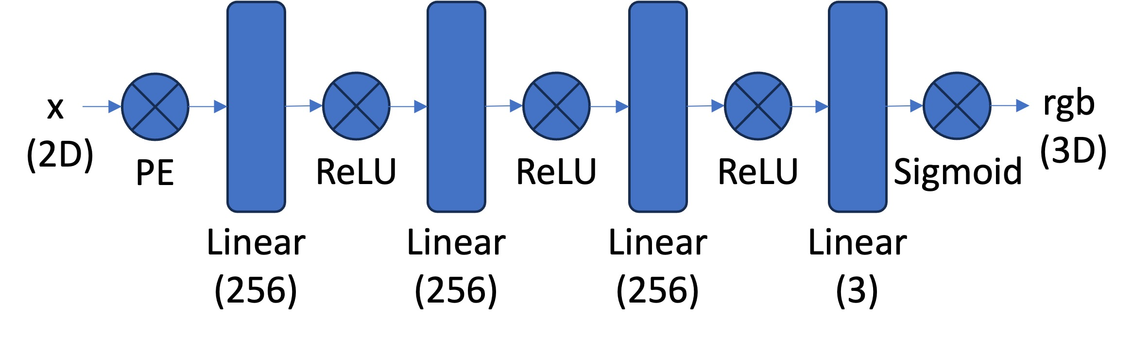
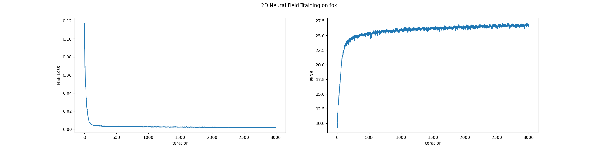
In 2D, a degenerated Neural Field is just a function \(F: (u, v) \mapsto (r, g, b)\) mapping image coordinates into rgb pixel values. I use the four layer MLP with 256 hidden dimensions (details shown below) to fit the Neural Field. The final Sigmoid activation ensures that the output is between 0 and 1. Since neural nets have inductive bias towards low frequency features, I use the sinusoidal positional encoding \(x \mapsto (x, \sin(2^0 \pi x), \cos(2^0 \pi x), ..., \sin(2^{L-1} \pi x), \cos(2^{L-1} \pi x))\) where \(L = 10\) (so the input is now a 42-dimensional vector). For fitting the fox picture below, I use Adam with \(lr=0.01\), batch size 10000 (pixels), and train for 3000 iterations. The training curve (reporting the MSE loss of the pixels and the Peak Signal-to-Noise Ratio \(PSNR = 10 \cdot \log_{10}(\frac{1}{MSE})\)), and the gradual improvement of the rendered image are shown below. The ground truth image is the rightmost image in the row.

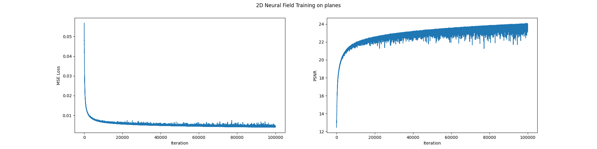
I also fit the Neural Field to the image of the Museum of Flight. I use 512 hidden dimensions instead of 256, use the Adam optimizer with \(lr=0.0001\), batch size 100000 (pixels), and train for 100000 iterations. The training curve and the gradual improvement of the rendered image are shown below. The ground truth image is the rightmost image in the row. We observe that this image is harder to fit than the fox image, possibly because it is of high resolution (the Meseum of Flight image is of resolution \(3024 \times 4032\) whereas the fox image is \(689 \times 1024\)).

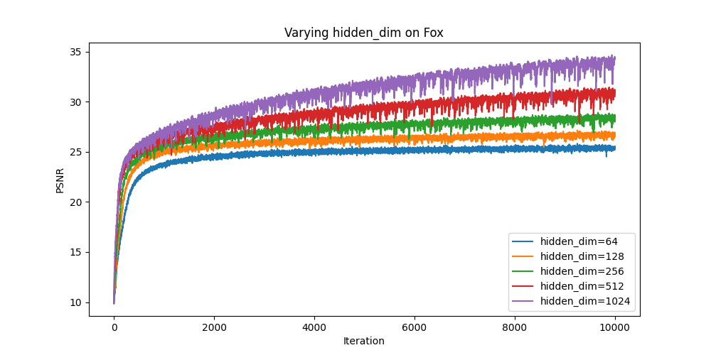
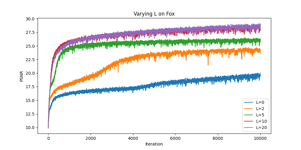
For the fox image, I try to vary the \(L\) (the number of positional encoding terms is \(2L+1\) for each pixel dimension) and the hidden dimensions of the MLP separately. To ensure convergence, I use a batch size of 10000 pixels, use Adam with \(lr=0.001\), 256 hidden dimensions and \(L = 10\) by default, 4 layers of MLP, and train for 10000 iterations. The training curves and the rendered images are shown below. We observe that when \(L\) is smaller than 5, the PSNR is relatively low. As \(L\) increases, the PSNR and the quality of the rendered images increases, but the difference between \(L = 10, 20\) are relatively small. This might be because some fourier features are necessary, but excessive fourier features with extremely high frequencies might not help neural network learning as much as their lower frequency counterparts. The PSNR and the quality of the rendered images increase as the hidden dimensions increase, since the expressive power of the MLP can be roughly proxied by the number of hidden dimensions, given they have the same depth.

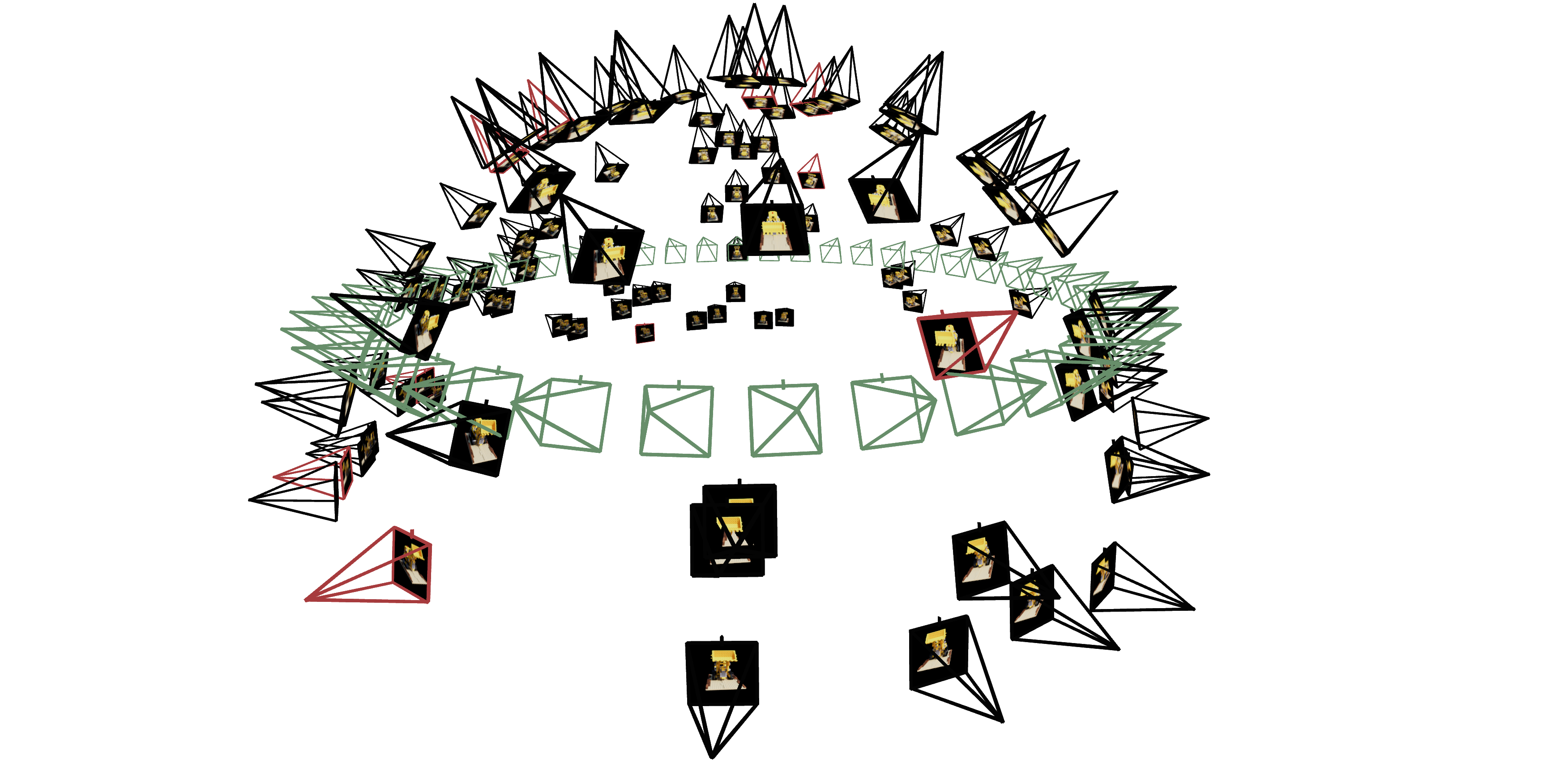
In 3D, a Neural Radiance Field parameterizes the 3D space with a neural network \(F: (x, y, z, \theta, \phi) \mapsto (r, g, b, \sigma)\) that maps spatial positions and view angles (during implementation we use a normalized view vector instead of angles) to rgb color and a density \(\sigma\). With this representation, we can use volumetric rendering to render the 2D pixel colors given any camera extrinsics. Concretely, we sample rays from the camera's projection center, through each pixel on the image plane, and denote the ray as \(\mathbf{r}(t)\) parameterized by a scalar \(t\). Then, if we let \(\sigma(\mathbf{r})\) be the density output and let \(\mathbf{c}(\mathbf{r}, \mathbf{d})\) be the color output of the Neural Radiance Field evaluated at position \(\mathbf{r}\), view direction \(\mathbf{d}\), the volumetric rendering equation gives us the rendered color as \[C(\mathbf{r}) = \int_{t_n}^{t_f} T(t) \sigma(\mathbf{r}(t)) \mathbf{c}(\mathbf{r}(t), \mathbf{d}) dt, T(t) = \exp(-\int_{t_n}^t \sigma(\mathbf{r}(s)) ds)\] Its discrete approximation is \[C(\mathbf{r}) = \sum_{i=1}^N T_i (1 - \exp(-\sigma_i \delta_i)) \mathbf{c}_i, T_i = \exp(-\sum_{j=1}^{i-1} \sigma_j \delta_j)\] where \(\delta_i\) is the spatial distance the i-th sampled point occupies. With images captured at different camera extrinsics (dataset shown below, black frames are training data, red frames are validation data, and green frames are test data), we can sample rays and train the Neural Radiance Field to render the actual pixels seen in the training set.

Creating Rays from Cameras

The given c2w (world-to-camera) matrices are rigid body transformation matrices in the form \[\begin{bmatrix} \mathbf{R} & \mathbf{t} \\ 0 & 1 \\ \end{bmatrix} \in \mathbb{R}^{4 \times 4}\] where \(\mathbf{R} \in \mathbb{R}^{3 \times 3}\) is an orthogonal matrix with determinant \(+1\) and \(\mathbf{t} \in \mathbb{R}^3\) is a translation vector. It transforms a point represented in the camera coordinate frame \((x_c, y_c, z_c, 1)\) in homogeneous coordinates to the world coordinate frame \((x_w, y_w, z_w, 1)\) in homogeneous coordinates through matrix multiplication \[\begin{bmatrix} x_w \\ y_w \\ z_w \\ 1 \\ \end{bmatrix} = \begin{bmatrix} \mathbf{R} & \mathbf{t} \\ 0 & 1 \\ \end{bmatrix} \begin{bmatrix} x_c \\ y_c \\ z_c \\ 1 \\ \end{bmatrix}\] By properties of rigid transformation matrices, we know \[\begin{bmatrix} \mathbf{R} & \mathbf{t} \\ 0 & 1 \\ \end{bmatrix}^{-1} = \begin{bmatrix} \mathbf{R}^T & -\mathbf{R}^T \mathbf{t} \\ 0 & 1 \\ \end{bmatrix}\] Combining these formulae, we can transform between the camera and world coordinate frames with either the c2w matrix or the w2c matrix (which is the inverse of the c2w matrix). The camera intrinsic matrix is \[K = \begin{bmatrix} f_x & 0 & o_x \\ 0 & f_y & o_y \\ 0 & 0 & 1 \\ \end{bmatrix}\] where \(f_x, f_y\) are the focal lengths of the camera, and \(o_x, o_y\) are the pixel offsets. It transforms points in the camera frame to pixel coordinates through s \[\begin{bmatrix} u \\ v \\ 1 \\ \end{bmatrix} = K \begin{bmatrix} x_c \\ y_c \\ z_c \\ \end{bmatrix}\] where \(s = z_c\) is the depth of the point in the camera frame. To sample rays (in the world frame), we first notice that the center of each camera is the \(\mathbf{t}\) translation vector in the corresponding c2w matrix. We can set the origin of the ray \(\mathbf{r}_o = \mathbf{t}\). Given the pixel coordinates \((u, v)\) and without loss of generality set the depth \(s = 1\), we can find the direction of the ray \(\mathbf{r}_d\) by transforming the pixel coordinates to the camera frame, and then to the world frame (denoted by \(\mathbf{X}_w\)). The direction of the ray is then \(\mathbf{r}_d = \frac{\mathbf{X}_w - \mathbf{r}_o}{||\mathbf{X}_w - \mathbf{r}_o||}\). We can then sample points along the ray by \(\mathbf{r}(t) = \mathbf{r}_o + t \mathbf{r}_d\).

Sampling

I create a dataloader that first converts all available training images and extrinsics to rays and their corresponding pixels. Each time we sample batch size number of rays (abstracting away the different images). To sample points along each ray, I linearly interpolate \(t\) from \(near=2\) to \(far=6\) and sample \(\mathbf{p} = \mathbf{r}_o + t \mathbf{r}_d \). During training, I also perturb each \(t\) by a random number between \(-0.5\) and \(0.5\) times the step size to avoid overfitting. I also implemented the coarse-to-fine sampling method, which I defer to later sections for duscussion.

Putting the Dataloading All Together

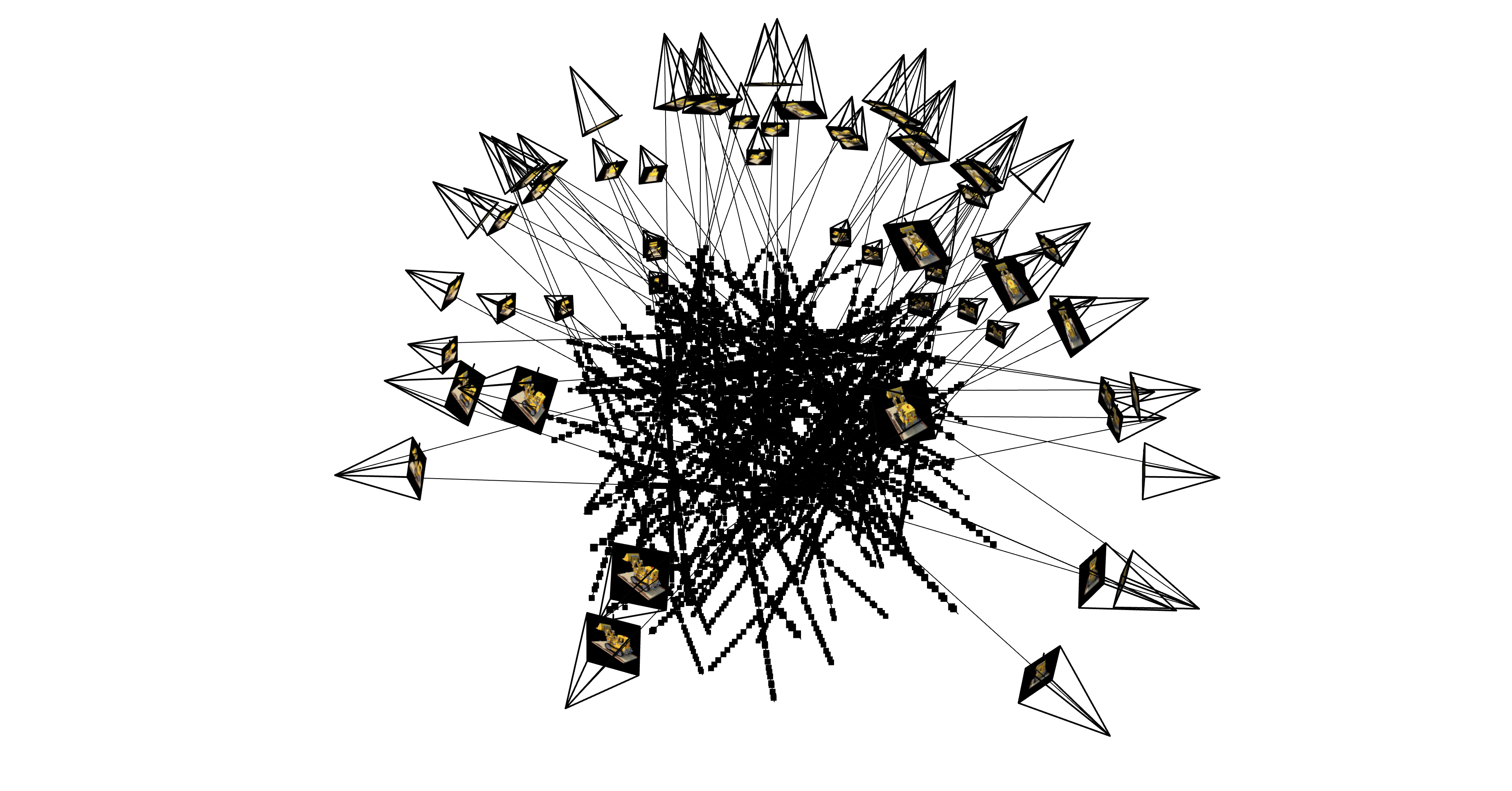
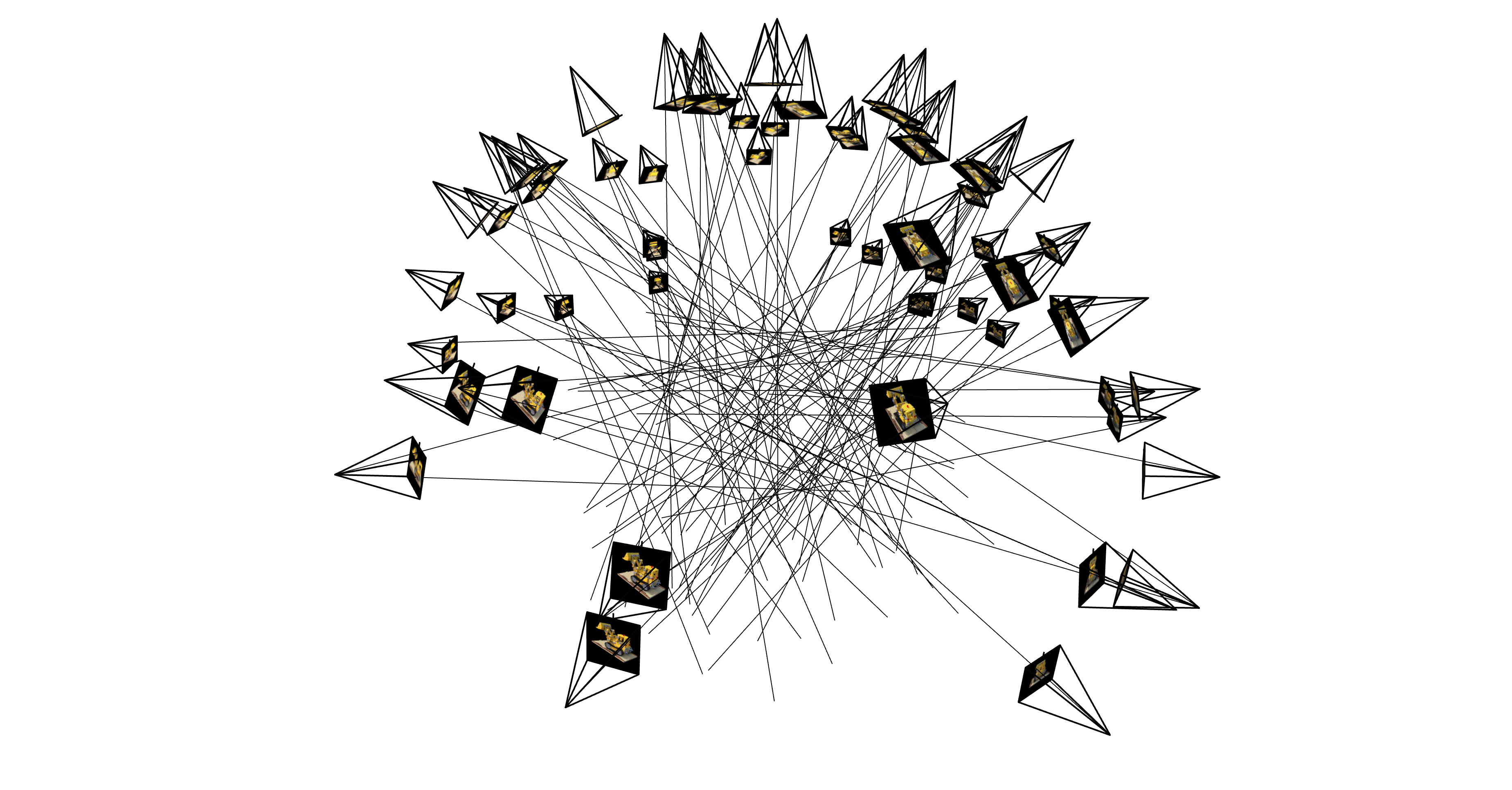
100 randomly sampled training images, rays, and 64 points along each ray are shown below (the first figure shows sampled points and the second figure does not). During training, this is one batch of data (except that the batch size is way larger than 100).

Neural Radiance Field

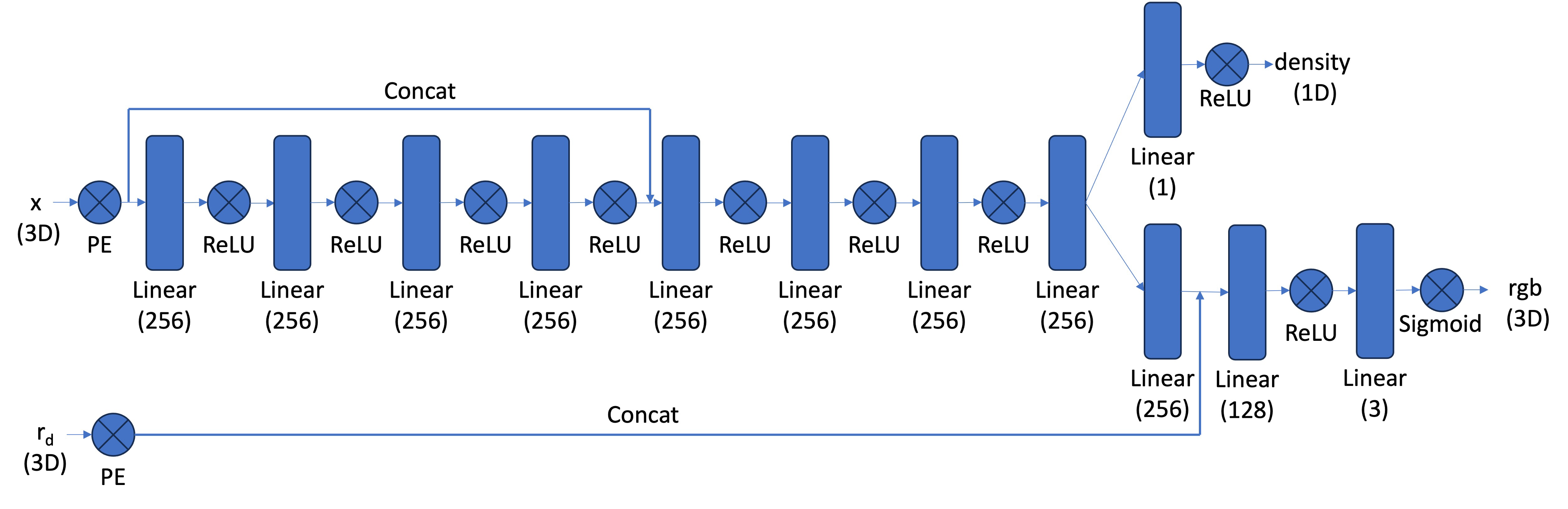
I implement a MLP Neural Radiance Field with a 7-layer backbone, and two heads for density and rgb separately. The final Sigmoid activation for the rgb head ensures that its output is within 0 and 1, and the final ReLU activation for the density head ensures its output is nonnegative. The detailed architecture is shown below. I use the same positional encoding as in the 2D case, and I choose \(L = 10\) for \(\mathbf{x}\) & \(L = 4\) for \(\mathbf{r}_d\).

Volumetric Rendering

As discussed above, the discrete version of the volumetric rendering formula is \[C(\mathbf{r}) = \sum_{i=1}^N T_i (1 - \exp(-\sigma_i \delta_i)) \mathbf{c}_i, T_i = \exp(-\sum_{j=1}^{i-1} \sigma_j \delta_j)\] We can use torch.cumsum to calculate \(T\), and the entire rendering procedure is differentiable.

Results (Vanilla Implementation)

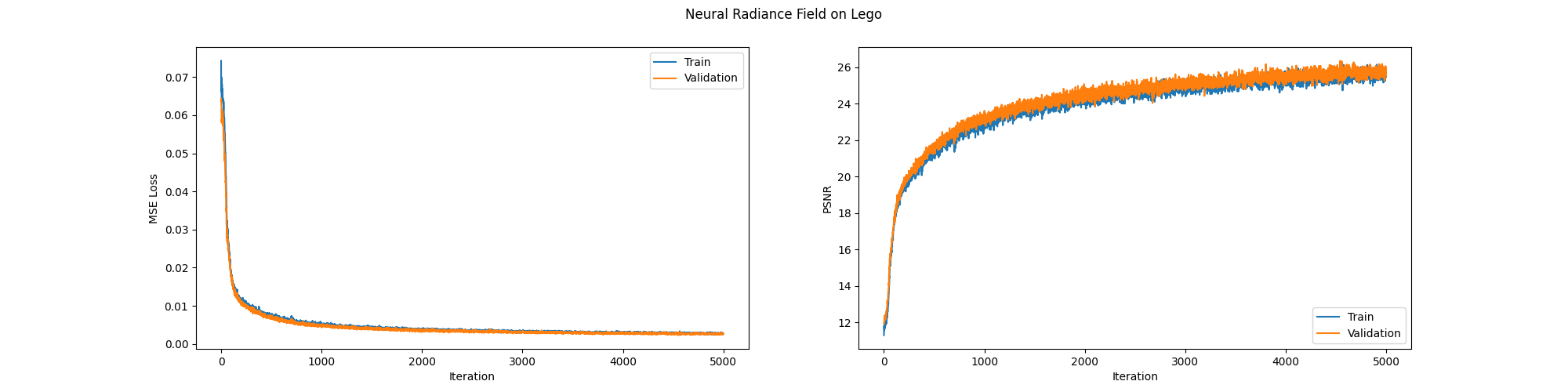
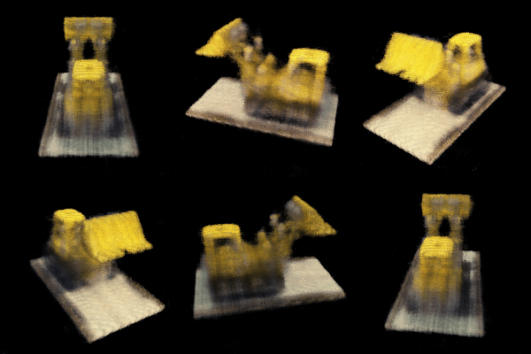
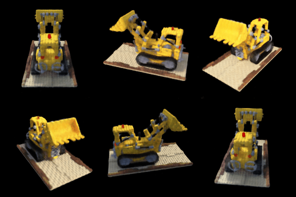
I use Adam with \(lr=0.0005\), sample 64 points along each ray, use a batch size of 10000 rays, and train for 5000 iterations. The training curve and the gradual improvement of the rendered image are shown below. The ground truth (which is in the validation dataset) image is the rightmost image in the row. The final PSNR is \(25.68\) (without coarse-to-fine sampling).

Below are rendered videos of the Lego scene with the camera extrinsics in the test set. The left video is rendered with 500 training iterations (which is of poor quality) and the right video is rendered with 5000 training iterations (which is of better quality but is still inferior to coarse-to-fine sampling).

Coarse-to-Fine Sampling & PSNR > 30

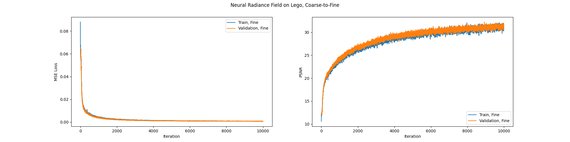
If we rewrite the discrete volumetric rendering formula as \[C(\mathbf{r}) = \sum_{i=1}^N w_i \mathbf{c}_i, w_i = T_i (1 - \exp(-\sigma_i \delta_i))\] We can see that the overall color is a weighted sum of the colors at the sampled points. Treating the weights as reletive importance and recalling each point is sampled uniformly from evenly spaced bins, we can see that the weights \(\frac{w_i}{\sum_{j} w_j}\) imposes a natural multinomial distribution on the bins. In coarse-to-fine sampling, we simultaneously optimize one "coarse" and one "fine" Neural Radiance Field (both have the architecture shown in the previous section). When rendering a pixel, we first "uniformly" (in the sense that we choose one point from each bin) samples 64 points (possibly with perturbation) and use the "coarse" Neural Radiance Field to render a "coarse" pixel color as described in the previous section. Then, we calcuate the weights \(w_i\) from the density output of the "coarse" Neural Radiance Field, and sample 128 additional points, first by sampling 128 bins according to the multinomial distribution defined bu the weights and then sample uniformly within each sampled bin to get the points. We combine the newly sampled 128 points and the 64 original points, and use volumetric rendering to calculate the fine pixel color with the "fine" Neural Radiance Field. During inference, we only use the "fine" rendered color, but during training we optimize the sum of the MSE loss of the "fine" rendered pixel color and the MSE loss of the "coarse" rendered pixel color. Since density serves as a proxy for importance, the coarse-to-fine sampling technique improves the sampling efficienty by paying more attention to important regions. I use the identical hyperparameters as the previous section, except that I use a batch size of 5000 rays and train for 10000 iterations. The training curve and the rendered videos of the Lego scene with the camera extrinsics in the test set are shown below. The final PSNR is \(31.32\), and the quality of the rendered video is significantly better than the vanilla implementation.

Rendering with Different Background Colors

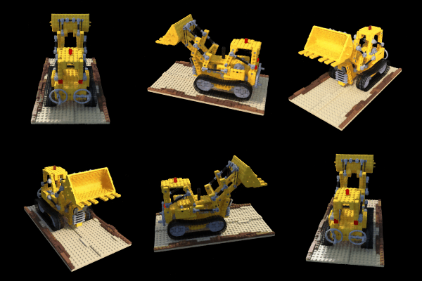
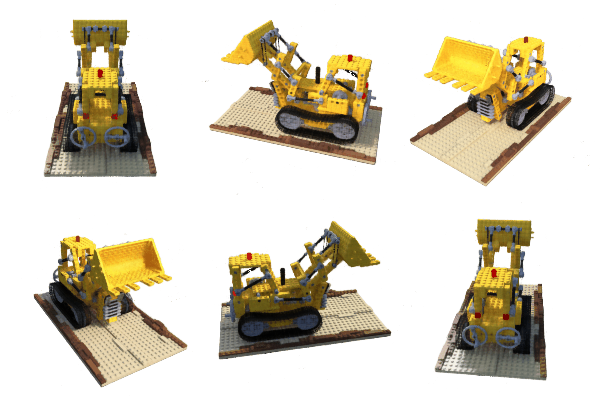
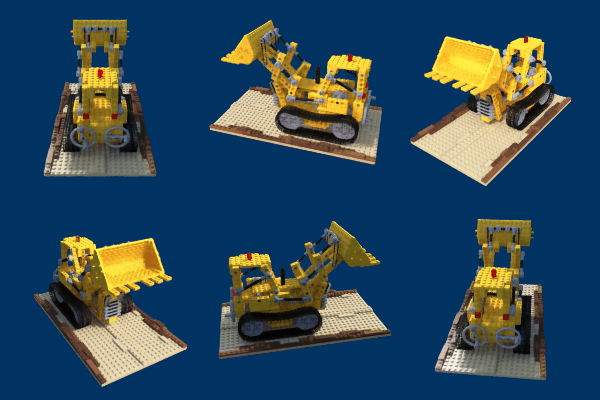
Intuitively, the background color is what is left of the densities. Concretely, we can extend the discrete volumetric rendering formula to \[C(\mathbf{r}) = \left(\sum_{i=1}^N T_i (1 - \exp(-\sigma_i \delta_i)) \mathbf{c}_i \right)+ \exp(-\sum_{j=1}^N \sigma_j \delta_j) \mathbf{c}_{\text{background}}, T_i = \exp(-\sum_{j=1}^{i-1} \sigma_j \delta_j)\] The addition of the background term ensures that the total weights sum up to 1: \(\left(\sum_{i=1}^N T_i (1 - \exp(-\sigma_i \delta_i)) \right) + \exp(\sum_{j=1}^N \sigma_j \delta_j) = 1\). When \(\mathbf{c}_{\text{background}} = (0, 0, 0)\), notice that the formula degenerates into the vanilla volumetric rendering formula and we have a black background. However, we now can set \(\mathbf{c}_{\text{background}}\) to any rgb value, and the rendered image will have the corresponding background color. Below are two examples (rendering with white and blue backgrounds).

Rendering Depth

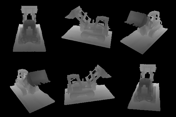
We can also render the depth map of the scene by rendering the distance of each pixel to the camera. Although changing the integrand/summand of the volumetric rendering formula should also work, I choose to use a simple cutoff strategy. I choose a cutoff between 0 and 1. For each pixel coordinate, I traverse through the corresponding ray starting from the camera center, and stop when \(T_i = \exp(-\sum_{j=1}^{i=1} \sigma_j \delta_j)\) is below \(1 - \text{cutoff}\), and set the pixel depth as the current distance to the camera center. Intuitively, we want the accumulated density to be at least as big as \(\text{cutoff}\) before we claim that we have reached the depth of the pixel. The reason for setting a nonzero cutoff is to filter out outliers, which has a nonzero density but should be considered as void visually. However a bigger cutoff might also filter out genuine non-void parts of the scene. Empirically I find \(0.3\) to be a reasonable cutoff, and the rendered depth video is shown below.